Example - Pen
Let us see a sample illustrating this process using a simple pipeline with a short mock autograph text, represented in Figure 1. Of course, that’s a totally unrealistic text, but it was created with the aim of including most of the operation types with a few words.
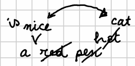
- Figure 1 - A mock autograph
The base text (version v0), written on the regular lines of the notebook, is just three words:
123456789
a red pen
Say that our interpretation defines the following operations starting from the base text, which is the one first written down on the regular notebook lines (after each operation I add the more formal representation of the operation in its DSL syntax):
- (
v0>v1): deletered+ space:"3x4- [*log="delete 'red '"]. - (
v1>v2): replacepenwithhat:7x3="hat" [*log="replace 'pen' with 'hat'"]. - (
v2>v3): replacehatwithcat:10x3="cat" [*log="replace 'hat' with 'cat'"]. - (
v3>v4): insertnice+ space beforecat:13+["nice " [*log="insert 'nice ' before 'cat'"]. - (
v4>v5): swapnicewithcat:16x4<>13x3 [*log="swap 'nice' with 'cat'"]. - (
v5>v6): insertis+ space beforenice:16+["is " [*log="insert 'is ' before 'nice'"].
These operations generate the following text versions:
v1:a penv2:a hatv3:a catv4:a nice catv5:a cat nicev6:a cat is nice
As usual, note that these are just the outputs of each operation. Every operation alters the text along the path leading from one staged version to the next one; so many of the outputs are just intermediate steps along this path. This is clearly the case especially when the output does not make sense, like in
v5. For instance, on the basis of external information here one might consider as staged versions justv4andv6. This is of course a matter of interpretation, within the constraints defined by the snapshot.
Tagging the image with numbers should make our interpretation more evident (Figure 2):
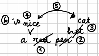
- Figure 2 - Tagged mock autograph
So, this is the essential data of our snapshot: a base text, and the operations affecting it. We now want to export this into a specific form of TEI, namely the scheme adopted by the Saba 1919 digital edition (which can be displayed in EVT 3).
There, for a given multiple-versions text (an epigram, a page, etc.):
- all the versions are inside an
appelement; - in
app, each version is inside alem(when the version is preferred by the editor) orrdgelement; - in
lem/rdg, amodcontains more metadata about the version (in attributes); - in
mod, we usedel,add, orsubstas customary in the TEI critical module.
Having defined both the start and the desired end of our transformation, let us now proceed with the export pipeline.
Stage 1
First, we use a tree builder to create a tree from the GVE snapshot. We then compose version trees into a “multi” tree, containing all the branches we want to export. Say we want only to export v4 and v6 assuming them as the staged versions, and that we want only trace features (dropping log features, in this example).
As remarked, when building the tree you can select the features you want in or out of the resulting nodes. Of course this depends on the annotations you will be using in generating the output. In this case we have no other metadata we are interested in; but there might be other cases where operations inject more metadata about e.g. other authors or revisors, ink types, etc. Any selected feature will be carried by its node, and pass through filters unless these are designed to affect them.
Also, we need to restore the deleted nodes into the exported trees, because we are going to need them in our desired TEI format. So, we just configure the builder accordingly via its options.
The dump for the linear tree built for v4 is:
+ ⯈ [1.1]
 + ⯈ [2.1] → #1: a
  + ⯈ [3.1] → #2:
   + ⯈ [4.1] → #16: n ($seg-out="fdf91da3b9 v3:v4 1", $seg-in="9dcb36963d v4:v5 1")
    + ⯈ [5.1] → #17: i ($seg-out="fdf91da3b9 v3:v4 2", $seg-in="9dcb36963d v4:v5 2")
     + ⯈ [6.1] → #18: c ($seg-out="fdf91da3b9 v3:v4 3", $seg-in="9dcb36963d v4:v5 3")
      + ⯈ [7.1] → #19: e ($seg-out="fdf91da3b9 v3:v4 4", $seg-in="9dcb36963d v4:v5 4")
       + ⯈ [8.1] → #20:   ($seg-out="fdf91da3b9 v3:v4 5")
        + ⯈ [9.1] → #3: r ($del="723a2d3720 v0:v1 1")
         + ⯈ [10.1] → #4: e ($del="723a2d3720 v0:v1 2")
          + ⯈ [11.1] → #5: d ($del="723a2d3720 v0:v1 3")
           + ⯈ [12.1] → #6:   ($del="723a2d3720 v0:v1 4")
            + ⯈ [13.1] → #7: p ($del="dc16589efc v1:v2 1")
             + ⯈ [14.1] → #8: e ($del="dc16589efc v1:v2 2")
              + ⯈ [15.1] → #9: n ($del="dc16589efc v1:v2 3")
               + ⯈ [16.1] → #10: h ($del="5292f1f888 v2:v3 1")
                + ⯈ [17.1] → #11: a ($del="5292f1f888 v2:v3 2")
                 + ⯈ [18.1] → #12: t ($del="5292f1f888 v2:v3 3")
                  + ⯈ [19.1] → #13: c ($seg2-in="9dcb36963d v4:v5 1", $seg-out="5292f1f888 v2:v3 1", $anchor="fdf91da3b9 v3:v4")
                   + ⯈ [20.1] → #14: a ($seg2-in="9dcb36963d v4:v5 2", $seg-out="5292f1f888 v2:v3 2")
                    - ■ [21.1] → #15: t ($seg2-in="9dcb36963d v4:v5 3", $seg-out="5292f1f888 v2:v3 3")
Here, each node is listed in a line, including its data payload after the right arrow: the node’s ID, its text value, and its optional features in brackets. Note that trace features, all starting with $, were automatically injected by operations.
Note that, as explained, trace feature values have always the form
OPID TAGIN:TAGOUT NR, whereOPID=operation ID,TAGIN=input version tag,TAGOUT=output version tag, andNR=ordinal number of the node in the segment selected by the operation. As for feature names,$seg-inrepresents a node selected by the operation as its input;$seg-outa node selected by the operation as its output;$dela deleted node. Names with$seg2...are the same, but refer to the second segment of a swap operation, which by definition deals with two distinct segments.
This is a linear tree, with a single branch starting from a blank node, and having a child node for each successive character. Here is the corresponding dump for v6:
+ ⯈ [1.1]
 + ⯈ [2.1] → #1: a
  + ⯈ [3.1] → #2:
   + ⯈ [4.1] → #16: n ($del="9dcb36963d v4:v5 1")
    + ⯈ [5.1] → #17: i ($del="9dcb36963d v4:v5 2")
     + ⯈ [6.1] → #18: c ($del="9dcb36963d v4:v5 3")
      + ⯈ [7.1] → #19: e ($del="9dcb36963d v4:v5 4")
       + ⯈ [8.1] → #3: r ($del="723a2d3720 v0:v1 1")
        + ⯈ [9.1] → #4: e ($del="723a2d3720 v0:v1 2")
         + ⯈ [10.1] → #5: d ($del="723a2d3720 v0:v1 3")
          + ⯈ [11.1] → #6:   ($del="723a2d3720 v0:v1 4")
           + ⯈ [12.1] → #7: p ($del="dc16589efc v1:v2 1")
            + ⯈ [13.1] → #8: e ($del="dc16589efc v1:v2 2")
             + ⯈ [14.1] → #9: n ($del="dc16589efc v1:v2 3")
              + ⯈ [15.1] → #10: h ($del="5292f1f888 v2:v3 1")
               + ⯈ [16.1] → #11: a ($del="5292f1f888 v2:v3 2")
                + ⯈ [17.1] → #12: t ($del="5292f1f888 v2:v3 3")
                 + ⯈ [18.1] → #13: c ($seg-out="5292f1f888 v2:v3 1", $anchor="fdf91da3b9 v3:v4", $seg2-in="9dcb36963d v4:v5 1")
                  + ⯈ [19.1] → #14: a ($seg-out="5292f1f888 v2:v3 2", $seg2-in="9dcb36963d v4:v5 2")
                   + ⯈ [20.1] → #15: t ($seg-out="5292f1f888 v2:v3 3", $seg2-in="9dcb36963d v4:v5 3")
                    + ⯈ [21.1] → #20:   ($seg-out="fdf91da3b9 v3:v4 5")
                     + ⯈ [22.1] → #21: i ($seg-out="56e0de97a8 v5:v6 1")
                      + ⯈ [23.1] → #22: s ($seg-out="56e0de97a8 v5:v6 2")
                       + ⯈ [24.1] → #23:   ($seg-out="56e0de97a8 v5:v6 3")
                        + ⯈ [25.1] → #13: c ($del="9dcb36963d v4:v5 1")
                         + ⯈ [26.1] → #14: a ($del="9dcb36963d v4:v5 2")
                          + ⯈ [27.1] → #15: t ($del="9dcb36963d v4:v5 3")
                           + ⯈ [28.1] → #16: n ($seg-out="fdf91da3b9 v3:v4 1", $seg-in="9dcb36963d v4:v5 1", $anchor="56e0de97a8 v5:v6")
                            + ⯈ [29.1] → #17: i ($seg-out="fdf91da3b9 v3:v4 2", $seg-in="9dcb36963d v4:v5 2")
                             + ⯈ [30.1] → #18: c ($seg-out="fdf91da3b9 v3:v4 3", $seg-in="9dcb36963d v4:v5 3")
                              - ■ [31.1] → #19: e ($seg-out="fdf91da3b9 v3:v4 4", $seg-in="9dcb36963d v4:v5 4")
So in the end we will have a “multi” tree with a blank root node having 2 branches for v4 and v6:
graph TB;

root --> v4-root
v4-root --> v4a[...]
root --> v6-root
v6-root --> v6a[...]
This tree can now enter the export pipeline.
Stage 2
The pipeline contains a single tree filter, the merge linear text tree filter. This will merge nodes into single nodes representing their text as a single, multiple-characters segment, according to the features we select.
In our example we are interested only in the trace features which help us define the text structure: $seg-out, $seg2-out, $del. This does not mean that other features will be dropped; it just means that they won’t be taken into consideration when delimiting the maximum extent of each segment according to its set of relevant features.
So, all the successive nodes sharing the same set of relevant features (here defined as $seg-out, $seg2-out, $del) will be merged into a single node, concatenating their characters into a single text segment.
Note that with “sharing the same set” we mean that, among the features defined as relevant, each merged node must have each feature name and value equal to the corresponding feature in another merged node. Yet, for values we can define filters to consider just a specific portion of them for the purpose of this comparison.
In our example, we are going to use a single feature value filter, represented by the regular expression
^([^ ]+).*$, replaced with$1. This means that we’re going to select only theOPIDoperation ID from the whole value of the trace features. This is required because otherwise we could not merge any nodes given that each of them has a different value forNR.
As already remarked, here we need to wrap this filter into a composite filter, because our tree really is just a wrapper for multiple trees, one per version. So, we are going to place in the pipeline a composite filter wrapping a linear merge filter. This will apply the linear merge filter to each sub-tree: v4 and v6.
The result of this filter can be summarized by a new dump (the two sub-trees have been separated by a blank line for more readability):
+ ⯈ [1.1]

 + ⯈ [2.1] →  (v=v4)
  + ⯈ [3.1] → #1: a
   + ⯈ [4.1] → #16: nice  ($seg-out="90da420ff9 v3:v4 1", $seg-in="f118ee1cd3 v4:v5 1", $seg-out="90da420ff9 v3:v4 2", $seg-in="f118ee1cd3 v4:v5 2", $seg-out="90da420ff9 v3:v4 3", $seg-in="f118ee1cd3 v4:v5 3", $seg-out="90da420ff9 v3:v4 4", $seg-in="f118ee1cd3 v4:v5 4", $seg-out="90da420ff9 v3:v4 5")
    + ⯈ [5.1] → #3: red  ($del="f3ac775e10 v0:v1 1", $del="f3ac775e10 v0:v1 2", $del="f3ac775e10 v0:v1 3", $del="f3ac775e10 v0:v1 4")
     + ⯈ [6.1] → #7: pen ($del="3b224463a2 v1:v2 1", $del="3b224463a2 v1:v2 2", $del="3b224463a2 v1:v2 3")
      + ⯈ [7.1] → #10: hat ($del="a915b9b07a v2:v3 1", $del="a915b9b07a v2:v3 2", $del="a915b9b07a v2:v3 3")
       - ■ [8.1] → #13: cat ($seg2-in="f118ee1cd3 v4:v5 1", $seg-out="a915b9b07a v2:v3 1", $anchor="90da420ff9 v3:v4", $seg2-in="f118ee1cd3 v4:v5 2", $seg-out="a915b9b07a v2:v3 2", $seg2-in="f118ee1cd3 v4:v5 3", $seg-out="a915b9b07a v2:v3 3")

 + ⯈ [2.2] →  (v=v6)
  + ⯈ [3.1] → #1: a
   + ⯈ [4.1] → #16: nice ($del="f118ee1cd3 v4:v5 1", $del="f118ee1cd3 v4:v5 2", $del="f118ee1cd3 v4:v5 3", $del="f118ee1cd3 v4:v5 4")
    + ⯈ [5.1] → #3: red  ($del="f3ac775e10 v0:v1 1", $del="f3ac775e10 v0:v1 2", $del="f3ac775e10 v0:v1 3", $del="f3ac775e10 v0:v1 4")
     + ⯈ [6.1] → #7: pen ($del="3b224463a2 v1:v2 1", $del="3b224463a2 v1:v2 2", $del="3b224463a2 v1:v2 3")
      + ⯈ [7.1] → #10: hat ($del="a915b9b07a v2:v3 1", $del="a915b9b07a v2:v3 2", $del="a915b9b07a v2:v3 3")
       + ⯈ [8.1] → #13: cat ($seg-out="a915b9b07a v2:v3 1", $anchor="90da420ff9 v3:v4", $seg2-in="f118ee1cd3 v4:v5 1", $seg-out="a915b9b07a v2:v3 2", $seg2-in="f118ee1cd3 v4:v5 2", $seg-out="a915b9b07a v2:v3 3", $seg2-in="f118ee1cd3 v4:v5 3")
        + ⯈ [9.1] → #20:   ($seg-out="90da420ff9 v3:v4 5")
         + ⯈ [10.1] → #21: is  ($seg-out="8f7c9ffd80 v5:v6 1", $seg-out="8f7c9ffd80 v5:v6 2", $seg-out="8f7c9ffd80 v5:v6 3")
          + ⯈ [11.1] → #13: cat ($del="f118ee1cd3 v4:v5 1", $del="f118ee1cd3 v4:v5 2", $del="f118ee1cd3 v4:v5 3")
           - ■ [12.1] → #16: nice ($seg-out="90da420ff9 v3:v4 1", $seg-in="f118ee1cd3 v4:v5 1", $anchor="8f7c9ffd80 v5:v6", $seg-out="90da420ff9 v3:v4 2", $seg-in="f118ee1cd3 v4:v5 2", $seg-out="90da420ff9 v3:v4 3", $seg-in="f118ee1cd3 v4:v5 3", $seg-out="90da420ff9 v3:v4 4", $seg-in="f118ee1cd3 v4:v5 4")
The following diagram summarizes the above dump (I applied the red color to the deleted nodes):

On passage, note that this defines a segment including only a space (between “cat” and “is”). This is the consequence of the design of the filter’s behavior, because that space refers to a different operation and thus has different metadata. Yet, the power of the pipeline approach is right in concatenating small pieces of reusable logic. Should we want to merge this space into the previous segment, we could just concatenate another filter which deals with whitespace-only segments and merges them following some specific logic.
Stage 3
Once we have our “multi” tree representing our staged versions, we can finally proceed to materialize this abstract structure into TEI markup.
As the tree contains multiple branches, one per sub-tree, we are going to use a composite “Saba” tree renderer. This will wrap a “Saba” tree renderer which, like most filters, just deals with a linear tree.
The logic of a composite renderer is more complex than that of a composite filter though, because the renderer might compose the partial renditions got from its inner component in unpredictable ways. So, we effectively have two distinct components: one is the single “Saba” tree renderer, which can be used also in isolation; another is the composed “Saba” tree renderer, which combines the results of the former into a single app element.
The single tree renderer essentially walks the linear branch down, and after adding a lem/rdg element with its child mod and some metadata, it inspects the trace features of each walked node:
- when it’s a delete, add a
subst/delbranch for replace or swap operations, or justdelfor other operation types. This is because we are going to represent the nodes removed by replace or swap to the left of the nodes which replaced them; and in this case we want to wrap both these groups into asubstelement representing the replacement operations as a deletion paired with an insertion. In both cases, thedelelement’s text will be represented by the deleted segment. - when it’s a
seg-out(orseg2-out) feature, add aninselement with the inserted segment as its text content. Then, if this has asubstancestor, pop XML elements until we reach the one belonging to the same operation of thedelelement. This ensures that we are properly wrapping each pair ofdel+insunder asubst. - when there is no feature, just add the text.
As you can see, the rendition logic here is minimal, because we are at the end of a pipeline where most of the work has already been completed in the previous stages.
The composite renderer just runs the inner renderer to each branch of the root tree node, adding each result to an app element. The result of this renderer for the two staged versions (v4 and v6) is reported below (I am pretty-printing the code here to make it more readable, even if in the real output no indentation is added inside mod):
<app xmlns="http://www.tei-c.org/ns/1.0">
  <rdg>
    <mod n="v4">a
      <ins source="oe43f114758">nice </ins>
      <del source="oda74a8a542">red </del>
      <subst source="o1218b2292d">
        <del>pen</del>
        <subst source="ob0f47c5e00">
          <del>hat</del>cat
        </subst>
      </subst>
    </mod>
  </rdg>
  <lem>
    <mod n="v6">a
      <subst source="od9ab6e69f9">
        <del>nice</del>
        <del source="oda74a8a542">red </del>
        <subst source="o1218b2292d">
          <del>pen</del>
          <subst source="ob0f47c5e00">
            <del>hat</del>cat
            <ins source="oe43f114758"></ins>
          </subst>
        </subst>
        <ins source="o951ad2d17c">is </ins>
        <subst source="od9ab6e69f9">
          <del>cat</del>
          <ins source="oe43f114758">nice</ins>
        </subst>
      </subst>
    </mod>
  </lem>
</app>
Note that this is a simplified rendition to keep the example readable; so we just added a @n attribute with the version tag to each mod, and a @source attribute linking to the corresponding operation. We could easily add much more data, and even think about rendering more features.
So, we got to the end of our pipeline: starting from a GVE snapshot, we ended up with a TEI document fragment which can be easily augmented by adding new filters in stage 4 (e.g. to wrap this result into a full TEI document template, add more metadata to the header, etc.). All the components along the pipeline have access to the rendering context, which keeps a shared state and allows to get data directly from the GVE model itself, and to a logging system, which provides diagnostic details about each rendition stage.